8. Estimating Fluxes at INST state
To estimate metabolic fluxes at the INST state, FreeFlux uses a nonlinear optimization approach that takes into account both metabolite concentrations and MDVs from multiple timepoints. The problem can be defined mathematically as follows:
Here, \({\bf{x}}_{sim}\) represents the simulated MDVs at all timepoints, and \({\bf{v}}_{sim}\) represents the simulated fluxes. Both are functions of the independent variable vector \(\bf{p}\), which includes free fluxes \(\bf{u}\) and concentrations \(\bf{c}\). \({\bf{x}}_{exp}\) and \({\bf{v}}_{exp}\) are the measurements of MDV and flux, respectively, and \({\bf{\Sigma }}_{{{\bf{x}}_{exp}}}^{ - 1}\) and \({\bf{\Sigma }}_{{{\bf{v}}_{exp}}}^{ - 1}\) are the inverses of the covariance matrix of measurements. \(\bf{N}\) is the null space of stoichiometric matrix of the network reactions, and \(\bf{T}\) denotes the matrix that transforms total fluxes to net fluxes.
8.1. Solving both the Fluxes and Concentrations
Similar to before, we start by building a metabolic model by reading the reactions from a file.
[1]:
from freeflux import Model

MODEL_FILE = 'path/to/reactions.tsv'

model = Model('demo')
model.read_from_file(MODEL_FILE)

ifit = model.fitter('inst')
Next, we specify the labeling strategy for the labeled substrates:
[2]:
ifit.set_labeling_strategy(
    'AcCoA',
    labeling_pattern = ['01', '11'],
    percentage = [0.25, 0.25],
    purity = [1, 1]
)   # call this method for each labeled substrate
The measured metabolite-derived isotopomer fractions (MDVs) and fluxes can be loaded one by one using set_measured_MDV and set_measured_flux, or all at once from files using set_measured_MDVs_from_file and set_measured_fluxes_from_file:
[3]:
MEASURED_MDV_FILE = 'path/to/measured_inst_MDVs.tsv'
MEASURED_FLUX_FILE = 'path/to/measured_fluxes.tsv'

ifit.set_measured_MDVs_from_file(MEASURED_MDV_FILE)
ifit.set_measured_fluxes_from_file(MEASURED_FLUX_FILE)
Next, we set the lower and upper bounds for the net fluxes and concentrations using set_flux_bounds and set_concentration_bounds, respectively:
[4]:
ifit.set_flux_bounds('all', bounds = [-100, 100])
ifit.set_concentration_bounds('all', bounds = [0.001, 10])
Note: 1. The upper bound should be great than the lower bound. Use set_measured_flux or set_measured_fluxes_from_file for equality assignment; 2. Bounds specified by set_concentration_bounds are not used as constraints in the optimization, it just defines the sampling range of the initial guess of concentrations; 3. By default, fluxes, concentrations and timepoints have the unit of \(\mu\)mol gCDW\(^{-1}\) s\(^{-1}\), \(\mu\)mol gCDW\(^{-1}\), and s,
respectively.
Finally, we solve for the fluxes and concentrations:
[5]:
ifit.prepare(n_jobs = 3)
res = ifit.solve(
    solver = 'ralg',
    ini_fluxes = None,
    fit_measured_fluxes = True
)
print(res.optimization_successful)
INST fitting [elapsed: 0:00:56]

True
The “fit_measured_fluxes” parameter in the solve method determines whether the measured fluxes are included in the optimization or not.
Currently, two methods are available to solve the fitting problem: the sequential least squares programming (solver=”slsqp”) and the r-algorithm with adaptive space dilation (solver=”ralg”, OpenOpt required). The two methods may have different performance on different models and input data. To use the r-algorithm solver, OpenOpt is required, and you can find more details on how to install it here.
The “ini_fluxes” argument is used to enter an initial guess of the fluxes, which can be derived from the last successful optimization. This argument takes a Pandas Series object or a .tsv/.xlsx file. A good initial guess can help with convergence. If None, the solve method will use a random initial guess sampled from the feasible region of fluxes estimated by flux variability analysis (FVA).
The “fit_measured_fluxes” argument determines whether the second flux item is included in the objective function of the above-formulated problem. Set this argument to True if exchange fluxes (e.g., substrate uptake rate, product secretion rate, or the specific cell growth) are measured and provided by set_measured_flux or set_measured_fluxes_from_file. In this case, the estimated fluxes have the same unit as the measured ones, which is \(\mu\)mol gCDW\(^{-1}\)
s\(^{-1}\) by default.
Additional arguments can be used to control the optimization process. For example, the “tol” and “max_iters” arguments can be used to set the tolerance level and maximum number of iterations for the solver, respectively. The “show_progress” argument can be set to True to display the time elapsed during the optimization.
The results of the optimization are stored in an InstFitResults object. The optimal objective value can be accessed through the opt_objective attribute of the object.
[6]:
res.opt_objective
[6]:
0.018
The optimal fluxes can be accessed by:
[7]:
print(res.opt_net_fluxes) # opt_total_fluxes for total fluxes
v1: 10.001
v2: 10.001
v3: 4.972
v4: 5.029
v5: 5.029
v6: 5.029
v7: 4.972
And the optimal concentration can be accessed by:
[8]:
print(res.opt_concentrations)
AKG: 0.281
Cit: 4.98
Fum: 0.141
Glu: 0.514
OAA: 2.246
Suc: 0.049
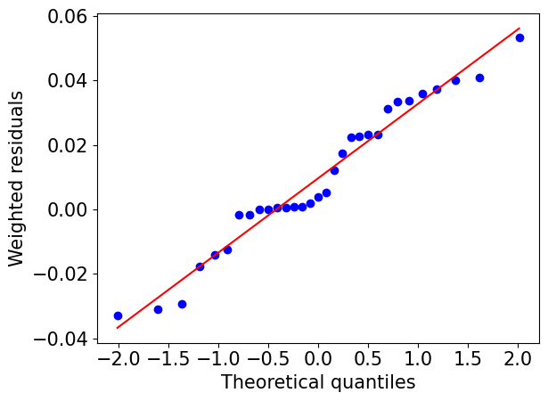
We can also use plot_normal_probability to check the goodness of fit:
[9]:
res.plot_normal_probability(show_fig = True, output_dir = None)
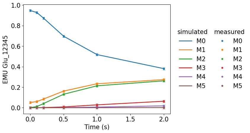
Comparison of the simulated and experimental measurements can be made by:
[10]:
res.plot_simulated_vs_measured_MDVs(show_fig = True, output_dir = None)
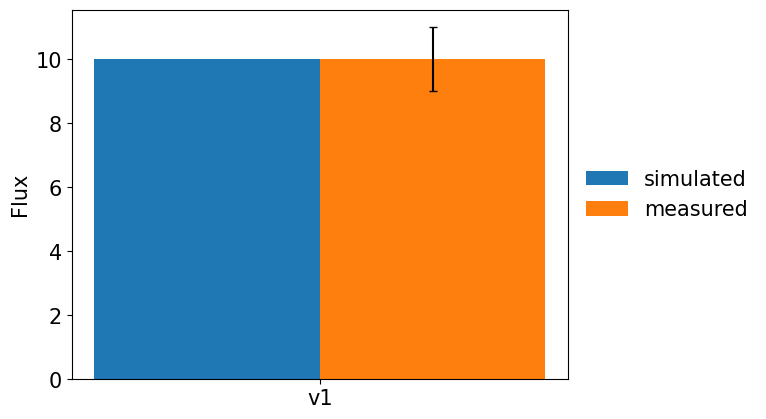
[11]:
res.plot_simulated_vs_measured_fluxes(show_fig = True, output_dir = None)
Symmetric confidence intervals of fluxes at convergence can be obtained using the estimate_confidence_intervals method:
[12]:
print(res.estimate_confidence_intervals(
    which = 'net',   # which = "total" for total fluxes
    confidence_level = 0.95
))
v1: [9.125, 10.876]
v2: [9.125, 10.876]
v3: [4.219, 5.725]
v4: [3.845, 6.213]
v5: [3.845, 6.213]
v6: [3.845, 6.213]
v7: [4.219, 5.725]
[13]:
print(res.estimate_confidence_intervals(which = 'conc', confidence_level = 0.95))
AKG: [0.0, 3.603]
Cit: [3.013, 6.946]
Fum: [0.0, 1138.422]
Glu: [0.0, 2.857]
OAA: [0.0, 972.684]
Suc: [0.0, 181.646]
We can evaluate the contribution of measurement variances (including all timepoints) to the uncertainty of estimated fluxes by calculating the contribution matrix:
[14]:
print(res.estimate_contribution_matrix(which = 'net')) # which = "total" for total fluxes
    Glu_12345_m0_0.1  Glu_12345_m1_0.1  Glu_12345_m2_0.1  Glu_12345_m3_0.1  \
v1          0.006657          0.001562          0.002262          0.000016
v2          0.006657          0.001562          0.002262          0.000016
v3          0.012128          0.002408          0.003313          0.000010
v4          0.000094          0.000004          0.000002          0.000024
v5          0.000094          0.000004          0.000002          0.000024
v6          0.000094          0.000004          0.000002          0.000024
v7          0.012128          0.002408          0.003313          0.000010

    Glu_12345_m4_0.1  Glu_12345_m5_0.1  Glu_12345_m0_0.2  Glu_12345_m1_0.2  \
v1      2.239544e-06      3.003782e-10          0.049795          0.015252
v2      2.239544e-06      3.003782e-10          0.049795          0.015252
v3      1.395488e-07      1.694144e-11          0.084663          0.015899
v4      1.805789e-06      2.380560e-10          0.000403          0.000123
v5      1.805789e-06      2.380560e-10          0.000403          0.000123
v6      1.805789e-06      2.380560e-10          0.000403          0.000123
v7      1.395488e-07      1.694144e-11          0.084663          0.015899

    Glu_12345_m2_0.2  Glu_12345_m3_0.2  ...  Glu_12345_m3_1.0  \
v1          0.023665          0.001707  ...          0.147273
v2          0.023665          0.001707  ...          0.147273
v3          0.021487          0.000233  ...          0.000035
v4          0.000420          0.001620  ...          0.082639
v5          0.000420          0.001620  ...          0.082639
v6          0.000420          0.001620  ...          0.082639
v7          0.021487          0.000233  ...          0.000035

    Glu_12345_m4_1.0  Glu_12345_m5_1.0  Glu_12345_m0_2.0  Glu_12345_m1_2.0  \
v1          0.020384          0.000204          0.142737          0.043837
v2          0.020384          0.000204          0.142737          0.043837
v3          0.000023          0.000002          0.407109          0.004165
v4          0.011793          0.000132          0.469267          0.038342
v5          0.011793          0.000132          0.469267          0.038342
v6          0.011793          0.000132          0.469267          0.038342
v7          0.000023          0.000002          0.407109          0.004165

    Glu_12345_m2_2.0  Glu_12345_m3_2.0  Glu_12345_m4_2.0  Glu_12345_m5_2.0  \
v1          0.017978          0.005100          0.000345          0.000342
v2          0.017978          0.005100          0.000345          0.000342
v3          0.007589          0.123542          0.015118          0.000143
v4          0.023875          0.076347          0.004156          0.000037
v5          0.023875          0.076347          0.004156          0.000037
v6          0.023875          0.076347          0.004156          0.000037
v7          0.007589          0.123542          0.015118          0.000143

          v1
v1  0.170514
v2  0.170514
v3  0.000466
v4  0.101747
v5  0.101747
v6  0.101747
v7  0.000466

[7 rows x 31 columns]
The sensitivities of estimated fluxes with respect to measurement perturbations (including all timepoints) can be obtained by:
[15]:
print(res.estimate_sensitivity(which = 'net')) # which = "total" for total fluxes
    Glu_12345_m0_0.1  Glu_12345_m1_0.1  Glu_12345_m2_0.1  Glu_12345_m3_0.1  \
v1         -3.369194          1.632079          1.963988         -0.164362
v2         -3.369194          1.632079          1.963988         -0.164362
v3         -3.912126          1.743226          2.044739          0.110744
v4          0.542932         -0.111147         -0.080751         -0.275106
v5          0.542932         -0.111147         -0.080751         -0.275106
v6          0.542932         -0.111147         -0.080751         -0.275106
v7         -3.912126          1.743226          2.044739          0.110744

    Glu_12345_m4_0.1  Glu_12345_m5_0.1  Glu_12345_m0_0.2  Glu_12345_m1_0.2  \
v1         -0.061796         -0.000716         -9.214526          5.099624
v2         -0.061796         -0.000716         -9.214526          5.099624
v3          0.013270          0.000146        -10.336268          4.479272
v4         -0.075066         -0.000862          1.121742          0.620352
v5         -0.075066         -0.000862          1.121742          0.620352
v6         -0.075066         -0.000862          1.121742          0.620352
v7          0.013270          0.000146        -10.336268          4.479272

    Glu_12345_m2_0.2  Glu_12345_m3_0.2  ...  Glu_12345_m3_1.0  \
v1          6.352281         -1.705824  ...        -15.846819
v2          6.352281         -1.705824  ...        -15.846819
v3          5.207194          0.542625  ...          0.211619
v4          1.145087         -2.248449  ...        -16.058438
v5          1.145087         -2.248449  ...        -16.058438
v6          1.145087         -2.248449  ...        -16.058438
v7          5.207194          0.542625  ...          0.211619

    Glu_12345_m4_1.0  Glu_12345_m5_1.0  Glu_12345_m0_2.0  Glu_12345_m1_2.0  \
v1         -5.895495         -0.590468        -15.600880          8.645712
v2         -5.895495         -0.590468        -15.600880          8.645712
v3          0.170868          0.051010         22.665844         -2.292551
v4         -6.066363         -0.641478        -38.266723         10.938263
v5         -6.066363         -0.641478        -38.266723         10.938263
v6         -6.066363         -0.641478        -38.266723         10.938263
v7          0.170868          0.051010         22.665844         -2.292551

    Glu_12345_m2_2.0  Glu_12345_m3_2.0  Glu_12345_m4_2.0  Glu_12345_m5_2.0  \
v1          5.536727          2.948962         -0.766712         -0.763809
v2          5.536727          2.948962         -0.766712         -0.763809
v3         -3.094699        -12.486040         -4.367789         -0.424765
v4          8.631426         15.435002          3.601078         -0.339044
v5          8.631426         15.435002          3.601078         -0.339044
v6          8.631426         15.435002          3.601078         -0.339044
v7         -3.094699        -12.486040         -4.367789         -0.424765

          v1
v1  0.170514
v2  0.170514
v3 -0.007671
v4  0.178185
v5  0.178185
v6  0.178185
v7 -0.007671

[7 rows x 31 columns]
Similarly, the with statement can also be used to perform flux estimation:
with model.fitter('inst') as ifit:
    ifit.set_labeling_strategy(
        'AcCoA',
        labeling_pattern = ['01', '11'],
        percentage = [0.25, 0.25],
        purity = [1,1]
    )
    ifit.set_measured_MDVs_from_file(MEASURED_MDVS)
    ifit.set_measured_fluxes_from_file(MEASURED_FLUXES)
    ifit.set_flux_bounds(
        'all',
        bounds = [-100, 100]
    )
    ifit.set_concentration_bounds(
        'all',
        bounds = [0.001, 10]
    )
    ifit.prepare(n_jobs = 3)
    res = ifit.solve(solver = 'ralg')
A more complex example of flux estimation at INST state using an Synechocystis model is provided in the script “tutorial_synechocystis_inst_estimation.py”
8.2. Dilution Parameter
Transient labeling of metabolites can be impeded by dilution effect. To account for it, we can add several special reactions to the network:
where A is the metabolite involved in metabolic reactions, Au is the metabolically inactive (unlabeled) fraction, and As is the pseudo-metabolite denoting the metabolites measured in samples. The zero coefficient in v1 and v2 guarantees that the additional metabolites will have no effect on the mass balance of network reactions. The flux values of the reactions could be arbitrary, but the ratio v2/(v1+v2) is determined by the labeling patterns of A, Au, and As, which is estimated as the dilution parameter.
Then, we need to tell the decomposer the unlabeled dilution source(s), i.e., “Au” in the above example by setting the argument “dilution_from = ‘Au’” in the prepare method.
8.3. Solving the Fluxes with Confidence Intervals
Uncertainties of fluxes and concentrations can be estimated using the Monte Carlo method. The following code demonstrates how to do this:
[16]:
model = Model('demo')
model.read_from_file(MODEL_FILE)

with model.fitter('inst') as ifit:
    ifit.set_labeling_strategy(
        'AcCoA',
        labeling_pattern = ['01', '11'],
        percentage = [0.25, 0.25],
        purity = [1,1]
    )
    ifit.set_measured_MDVs_from_file(MEASURED_MDV_FILE)
    ifit.set_measured_fluxes_from_file(MEASURED_FLUX_FILE)
    ifit.set_flux_bounds(
        'all',
        bounds = [-100, 100]
    )
    ifit.set_concentration_bounds(
        'all',
        bounds = [0.001, 10]
    )
    ifit.prepare(n_jobs = 30)
    res = ifit.solve_with_confidence_intervals(
        n_runs = 30,
        n_jobs = 3
    )
INST fitting with CIs [elapsed: 0:07:49]
Note: For the estimation of CIs for large-sized models, we strongly recommend running with parallel jobs. One can achieve this by setting the ‘n_jobs’ argument of the solve_with_confidence_intervals method to a value greater than 1.
[17]:
print(res.estimate_confidence_intervals(
    which = 'net',   # which = "total" for total fluxes
    confidence_level = 0.95
))
v1: [8.078, 10.78]
v2: [8.078, 10.78]
v3: [2.102, 5.724]
v4: [3.605, 8.557]
v5: [3.605, 8.557]
v6: [3.605, 8.557]
v7: [2.102, 5.724]
[18]:
print(res.estimate_confidence_intervals(which = 'conc', confidence_level = 0.95))
AKG: [0.0, 1.277]
Cit: [0.001, 5.554]
Fum: [0.0, 1.23]
Glu: [0.0, 3.375]
OAA: [0.001, 2.916]
Suc: [0.0, 2.489]
For a more complex example of flux estimation with CIs of a Synechocystis model, please refer to the script “tutorial_synechocystis_inst_estimation.py”