6. Estimating Fluxes at Steady State
To estimate metabolic fluxes at steady state, we use nonlinear optimization to minimize the difference between the simulated and measured labeling patterns when the system reaches a stable status, both metabolically and isotopically. The problem can be formulated as follows:
Here, \({\bf{x}}_{sim}\) and \({\bf{v}}_{sim}\) are simulated MDVs and fluxes, respectively, both the functions of free flux \(\bf{u}\). \({\bf{x}}_{exp}\) and \({\bf{v}}_{exp}\) are the measured labeling patterns and fluxes, and \({\bf{\Sigma }}_{{{\bf{x}}_{exp}}}^{ - 1}\) and \({\bf{\Sigma }}_{{{\bf{v}}_{exp}}}^{ - 1}\) are the inverses of the covariance matrix of measurements. \(\bf{N}\) is the null space of the stoichiometric matrix of the network reactions, and \(\bf{T}\) is the matrix that transforms total fluxes to net fluxes.
6.1. Solving the Fluxes
We will demonstrate the process using a toy model. First, we build the model by reading from the file:
[1]:
from freeflux import Model

MODEL_FILE = 'path/to/reactions.tsv'

model = Model('demo')
model.read_from_file(MODEL_FILE)

fit = model.fitter('ss')
Next, we specify the labeling strategy:
[2]:
fit.set_labeling_strategy(
    'AcCoA',
    labeling_pattern = ['01', '11'],
    percentage = [0.25, 0.25],
    purity = [1, 1]
)   # call this method for each labeled substrate
We can set the measurements using set_measured_MDV for MDV and set_measured_flux for flux (if any). To input a set of measurements, we can load from files using set_measured_MDVs_from_file and set_measured_fluxes_from_file methods. We assume here that the measured fluxes are net ones since total fluxes are not typically measurable:
[3]:
MEASURED_MDV_FILE = 'path/to/measured_MDVs.tsv'
MEASURED_FLUX_FILE = 'path/to/measured_fluxes.tsv'

fit.set_measured_MDVs_from_file(MEASURED_MDV_FILE)
fit.set_measured_fluxes_from_file(MEASURED_FLUX_FILE)
We can then set the lower and upper bounds of net fluxes:
[4]:
fit.set_flux_bounds(
    'all',   # "all" denotes all fluxes. use reaction ID for specific flux
    bounds = [-100, 100]
)
Note: The upper bound should be great than the lower bound. Use set_measured_flux or set_measured_fluxes_from_file for equality assignment.
Finally, we can solve for the fluxes:
[5]:
fit.prepare(n_jobs = 3)
res = fit.solve(
    solver = 'slsqp',
    ini_fluxes = None,
    fit_measured_fluxes = True
)
print(res.optimization_successful)
fitting [elapsed: 0:00:01]
True
Currently, FreeFlux offers two methods to solve the fitting problem: sequential least squares programming (solver = “slsqp”) and the r-algorithm with adaptive space dilation (solver = “ralg”). To use the r-algorithm solver, OpenOpt is required, and you can find more details on how to install it here.
The argument “ini_fluxes” is used to input an initial guess for the fluxes, which can be obtained from the last successful optimization. This argument takes a Pandas Series object or a .tsv/.xlsx file. A good initial guess can help with convergence. If you do not provide an initial guess, the solver will generate a random initial guess sampled from the feasible region of fluxes estimated by flux variability analysis (FVA).
The argument “fit_measured_fluxes” determines whether the second flux item is included in the objective function of the above-formulated problem. Set this argument to True if you have measured exchange fluxes, such as substrate uptake rate, product secretion rate, or specific cell growth, and provided them with set_measured_flux or set_measured_fluxes_from_file. In this case, the estimated fluxes will have the same unit as the measured ones, which are typically mmol gCDW\(^{-1}\)
h\(^{-1}\) or \(\mu\)mol gCDW\(^{-1}\) s\(^{-1}\). If you do not provide any measured flux, you can still provide a substrate uptake rate and fix its value at 100. In this case, the estimated fluxes will have relative values normalized to the substrate uptake rate.
Other arguments such as “tol” and “max_iters” control when the optimization stops, and “show_progress” controls whether to display the time elapsed during the optimization.
After optimization, the results are stored in the FitResults object, and the optimal objective can be accessed using the opt_objective attribute:
[6]:
print(res.opt_objective)
0.002
You can access the optimal net and total fluxes using the opt_net_fluxes and opt_total_fluxes attributes:
[7]:
print(res.opt_net_fluxes)
v1: 10.0
v2: 10.0
v3: 4.993
v4: 5.007
v5: 5.007
v6: 5.007
v7: 4.993
[8]:
print(res.opt_total_fluxes)
v1: 10.0
v2: 10.0
v3: 4.993
v4: 5.007
v5: 5.007
v6_f: 69.119
v6_b: 64.112
v7: 4.993
You can check the goodness of fit using the normal probability plot of weighted residuals. You can generate this plot using the following command:
[9]:
res.plot_normal_probability(show_fig = True, output_dir = None)
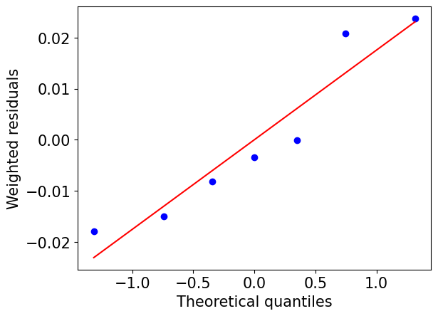
A good fit is indicated by the residuals closely following the red line, which represents a normal distribution.
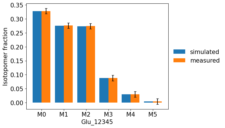
We can also compare the simulated and experimental measurements by plotting them together using the command:
[10]:
res.plot_simulated_vs_measured_MDVs(show_fig = True, output_dir = None)
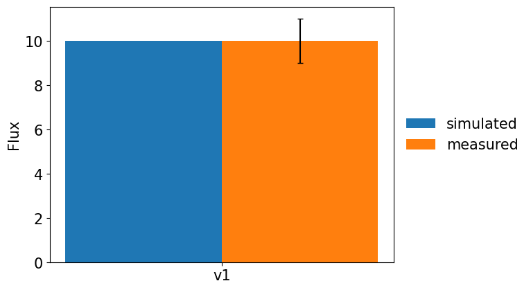
[11]:
res.plot_simulated_vs_measured_fluxes(show_fig = True, output_dir = None)
To obtain symmetric confidence intervals of net or total fluxes at convergence, you can use the estimate_confidence_intervals method:
[12]:
print(res.estimate_confidence_intervals(
    which = 'net',   # which = "total" for total fluxes
    confidence_level = 0.95
))
v1: [8.758, 11.242]
v2: [8.758, 11.242]
v3: [4.309, 5.677]
v4: [4.321, 5.693]
v5: [4.321, 5.693]
v6: [4.321, 5.693]
v7: [4.309, 5.677]
You can evaluate the contribution of measurement variances to the uncertainty of estimated fluxes by calculating the contribution matrix using the get_contribution_matrix method:
[13]:
print(res.estimate_contribution_matrix(which = 'net')) # which = "total" for total fluxes
    Glu_12345_m0  Glu_12345_m1  Glu_12345_m2  Glu_12345_m3  Glu_12345_m4  \
v1  2.193959e-29  4.692641e-29  6.652732e-29  1.992930e-29  3.961689e-30
v2  2.136664e-29  4.693636e-29  6.660495e-29  2.158797e-29  4.004388e-30
v3  1.252988e-01  2.058794e-04  2.293547e-03  4.182729e-02  8.895606e-03
v4  1.247228e-01  2.049330e-04  2.283004e-03  4.163501e-02  8.854712e-03
v5  1.247228e-01  2.049330e-04  2.283004e-03  4.163501e-02  8.854712e-03
v6  1.247228e-01  2.049330e-04  2.283004e-03  4.163501e-02  8.854712e-03
v7  1.252988e-01  2.058794e-04  2.293547e-03  4.182729e-02  8.895606e-03

    Glu_12345_m5        v1
v1  1.194661e-31  1.000000
v2  1.224363e-31  1.000000
v3  4.665391e-04  0.821012
v4  4.643944e-04  0.821835
v5  4.643944e-04  0.821835
v6  4.643944e-04  0.821835
v7  4.665391e-04  0.821012
we can also calculate the sensitivities of estimated fluxes to measurement perturbations using the following command:
[14]:
print(res.estimate_sensitivity(which = 'net')) # which = "total" for total fluxes
    Glu_12345_m0  Glu_12345_m1  Glu_12345_m2  Glu_12345_m3  Glu_12345_m4  \
v1 -4.683972e-13 -6.850286e-13 -8.156428e-13 -4.464224e-13 -1.990399e-13
v2 -4.622406e-13 -6.851011e-13 -8.161186e-13 -4.646285e-13 -2.001097e-13
v3  1.950560e+01  7.906644e-01 -2.639001e+00 -1.126978e+01 -5.197248e+00
v4 -1.950560e+01 -7.906644e-01  2.639001e+00  1.126978e+01  5.197248e+00
v5 -1.950560e+01 -7.906644e-01  2.639001e+00  1.126978e+01  5.197248e+00
v6 -1.950560e+01 -7.906644e-01  2.639001e+00  1.126978e+01  5.197248e+00
v7  1.950560e+01  7.906644e-01 -2.639001e+00 -1.126978e+01 -5.197248e+00

    Glu_12345_m5        v1
v1 -3.456387e-14  1.000000
v2 -3.499090e-14  1.000000
v3 -1.190227e+00  0.499299
v4  1.190227e+00  0.500701
v5  1.190227e+00  0.500701
v6  1.190227e+00  0.500701
v7 -1.190227e+00  0.499299
The with statement can also be used to perform flux estimation:
[15]:
with model.fitter('ss') as fit:
    fit.set_labeling_strategy(
        'AcCoA',
        labeling_pattern = ['01', '11'],
        percentage = [0.25, 0.25],
        purity = [1, 1]
    )
    fit.set_measured_MDVs_from_file(MEASURED_MDV_FILE)
    fit.set_measured_fluxes_from_file(MEASURED_FLUX_FILE)
    fit.prepare(n_jobs = 3)
    res = fit.solve(
        solver = 'slsqp',
        ini_fluxes = None,
        fit_measured_fluxes = True
    )
print(res.optimization_successful)
fitting [elapsed: 0:00:01]
True
A more complex example of steady state fitting using an E. coli model is provided in the script “tutorial_ecoli_steady_state_estimation.py”
6.2. Dilution Parameter
In some cases, the fractional labeling (13C enrichment) of certain metabolites, such as amino acids, can be significantly lower than that of other metabolites. This could be due to the presence of unlabeled fractions introduced from the inoculum, inactive pool or media. To better fit the data, dilution parameters need to be added to the network.
For instance, we can add the following three reactions to account for the dilution effect of a metabolite A with three C atoms:
Here, A represents the metabolite involved in metabolic reactions, Au represents the metabolically inactive (unlabeled) fraction, and As represents the pseudo-metabolite denoting the metabolite measured in samples. The zero coefficient in v1 and v2 ensures that the additional metabolites will have no effect on the mass balance of network reactions. The flux values of the reactions can be arbitrary, but the ratio v2/(v1+v2) is determined by the labeling patterns of A, Au, and As, and is estimated as the dilution parameter. These additional reactions are useful in accounting for the dilution effect of measured metabolites, such as amino acids. For unmeasured metabolites, such as CO\(_2\), only one reaction is needed:
v1: 0Au(abc) \(\rightarrow\) 0A(abc)
The zero coefficient on both sides excludes the reaction from mass balance, leaving it only to EMU decomposition.
To inform the decomposer about the unlabeled dilution source(s), i.e., “Au” in the above example, we can set the argument “dilution_from = ‘Au’” in the prepare method.
6.3. Solving the Fluxes with Confidence Intervals
In some cases, it is important to assess the uncertainty in estimated fluxes by calculating confidence intervals (CIs). FreeFlux utilizes the Monte Carlo method to estimate CIs. The commands for estimating fluxes with CIs are similar to those for flux estimation, except the method solve_with_confidence_intervals is used instead.
[16]:
with model.fitter('ss') as fit:
    fit.set_labeling_strategy(
        'AcCoA',
        labeling_pattern = ['01', '11'],
        percentage = [0.25, 0.25],
        purity = [1, 1]
    )
    fit.set_flux_bounds(
        'all',
        bounds = [-100, 100]
    )
    fit.set_measured_MDVs_from_file(MEASURED_MDV_FILE)
    fit.set_measured_fluxes_from_file(MEASURED_FLUX_FILE)
    fit.prepare(n_jobs = 3)
    res = fit.solve_with_confidence_intervals(
        n_runs = 90,
        n_jobs = 3
    )
print(res.estimate_confidence_intervals(
    which = 'net',
    confidence_level = 0.95
))
fitting with CIs [elapsed: 0:00:21]

v1: [8.487, 11.602]
v2: [8.487, 11.602]
v3: [4.195, 6.155]
v4: [4.002, 5.806]
v5: [4.002, 5.806]
v6: [4.002, 5.806]
v7: [4.195, 6.155]
Note: For the estimation of CIs for large-sized models, we strongly recommend running with parallel jobs. One can achieve this by setting the ‘n_jobs’ argument of the solve_with_confidence_intervals method to a value greater than 1.
A more complex example of estimating flux CIs of an E. coli model is provided in the script “tutorial_ecoli_steady_state_estimation.py”